
Driving a viewer from Python#
A viewer on your screen takes commands from Python as well as from your mouse. Set the stretch, move to a galaxy, collapse a cube’s planes, then read numbers back: statistics of regions, pixel values, a profile, the shape of a star, the brightest stars in the image, or a picture of the view as it is. Each change shows in the viewer as if you had made it with its own controls, so Ctrl+Z there undoes it. A notebook viewer, a pop-up window and a view open in VS Code or the desktop app all have the same methods.
Changing how it looks#
Open a viewer as usual and keep what pc.show returns. The examples here use the sample star field
with its galaxy.
import pixel_clarity as pc

v = pc.show("image.fits", height=560)
set_display changes how the image is drawn, as the toolbar would: the colormap, the scale
function and the limits here, and also contrast and bias, Auto enhance, binning, smoothing,
contours, the coordinate grid and the scale bar. Only what you give changes. It answers with the
display as it is afterwards, the limits worked out as numbers:
v.set_display(colormap="inferno", scale="asinh", limits="99.5")
{'display': {'colormap': 'inferno',
  'scale': 'asinh',
  'limits': '99.5',
  'lo': 86.166,
  'hi': 460.298}}
set_view moves the view. A position is an image pixel as in a .reg file ((x, y), counted
from 1, x to the right and y up), an astropy SkyCoord, or text such as
"10:00:22.7 +02:11:42"; the zoom is screen pixels per image pixel, or "fit". It also turns
the view (rotation, north_up), picks another array of the file, a frame of a cube or a
detector of a mosaic. snapshot() gives the view as it is on screen, as PNG bytes, which IPython
shows as a picture:
from IPython.display import Image

v.set_view(center=(981, 641), zoom=1)   # the galaxy, one screen pixel for each image pixel
v.set_display(grid=True)                # and a grid of right ascension and declination
Image(v.snapshot())
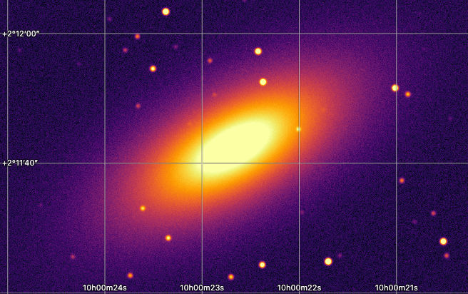
The viewer above is the view as pc.show opened it; the picture is the same view after the two
commands. snapshot("view.png") writes the picture to a file instead, and max_size sets its
longer side (1024 pixels at most by default). For a picture of the whole image at full
resolution, use save_png (see Saving pictures).
Reading values#
The commands that read from the view answer with plain Python: dictionaries, lists and numbers, with the image’s unit and, where the image has a WCS, sky positions beside pixel ones.
region_stats measures a region without drawing it. Give it as DS9 region text, a regions
object or a region file, in pixels or on the sky. Here a circle of radius 1.5″ around a bright
star:
stats = v.region_stats('fk5; circle(150.081879, 2.191928, 1.5")')
stats[0]
{'image': 'circle(1392.617,535.829,13.6364) # color=green',
 'sky': 'circle(150.081879,2.191928,1.5") # color=green',
 'n': 584,
 'sum': 94006.9,
 'mean': 160.971,
 'median': 102.708,
 'std': 197.67,
 'min': 82.3431,
 'max': 1482.04,
 'centroid': {'x': 1392.632,
  'y': 535.843,
  'ra': 150.0818785,
  'dec': 2.1919284},
 'unit': 'DN/s'}
You get the number of pixels, their sum, mean, median, standard deviation, minimum and maximum,
the centroid, and the AB magnitude where the file gives a flux scale. pixel_values reads the
pixels around a position, here a 3 × 3 square on the same star:
px = v.pixel_values((1393, 536), size=3)
px["rows"]
[[1232.316, 1263.4, 1023.455],
 [1435.731, 1482.036, 1212.188],
 [1336.475, 1371.942, 1127.778]]
The rows run from the top of the square down, as the view shows them; px["x"] and px["y"]
give the pixel coordinates of its corners.
examine_star fits the star nearest a position (an elliptical Gaussian, the sky measured in a
ring around it) and gives its center, FWHM, ellipticity, peak, sky and flux:
star = v.examine_star("10:00:19.65 +02:11:31.0")
star["center"], star["fwhm_arcsec"], star["flux"]
({'x': 1392.617, 'y': 535.816, 'ra': 150.081879, 'dec': 2.1919276},
 0.5177,
 35421.1)
profile gives the values along a line from one position to another, each point the mean (or
stat="median", "sum") across width pixels. Here 200 pixels across the galaxy’s core:
cut = v.profile((881, 641), (1081, 641), width=5)
peak = max(cut["values"])
cut["distance_arcsec"][cut["values"].index(peak)], peak
(11, 3037.11)
find_stars lists the brightest stars (and other compact sources) of the image, brightest first,
each measured as examine_star measures it. The search runs next to the data at full
resolution, not in the browser, so it works on images far larger than the view:
import pandas as pd

found = v.find_stars(8)
pd.DataFrame(found["stars"])
| x | y | ra | dec | flux | peak | fwhm_px | fwhm_arcsec | ellipticity | |
|---|---|---|---|---|---|---|---|---|---|
| 0 | 980.996 | 640.999 | 150.094465 | 2.195142 | 2379800 | 1744.1 | 23.10 | 2.550 | 0.380000 |
| 1 | 1442.217 | 1273.329 | 150.080362 | 2.214463 | 52680 | 2097.7 | 4.71 | 0.518 | 0.000650 |
| 2 | 1113.669 | 481.080 | 150.090409 | 2.190255 | 52047 | 2065.9 | 4.71 | 0.518 | 0.002100 |
| 3 | 879.357 | 1037.582 | 150.097573 | 2.207259 | 48244 | 1923.1 | 4.71 | 0.518 | 0.002200 |
| 4 | 885.885 | 831.230 | 150.097374 | 2.200954 | 45717 | 1824.2 | 4.71 | 0.518 | 0.000091 |
| 5 | 1308.939 | 1359.520 | 150.084437 | 2.217096 | 44852 | 1779.3 | 4.71 | 0.518 | 0.002300 |
| 6 | 1578.974 | 1263.353 | 150.076180 | 2.214158 | 44551 | 1772.4 | 4.71 | 0.518 | 0.001700 |
| 7 | 1532.322 | 1182.843 | 150.077607 | 2.211698 | 43456 | 1738.9 | 4.70 | 0.517 | 0.002900 |
The galaxy’s core is the brightest compact thing here, so it comes first; its FWHM of over 20
pixels sets it apart from the stars, which found["median_fwhm_px"] puts at about 4.7. region=
searches only inside a region, and min_sigma sets how far above its local background a star
must stand (5 by default).
Regions on the view#
Regions you draw in the viewer, and those added with add_regions, are measured all at once by
region_stats() without a region:
v.add_regions("image; circle(1392.6, 535.8, 12) # text={star A}")
[(r["image"], r["n"], r["mean"]) for r in v.region_stats()]
[('circle(1392.6,535.8,12) # color=green text={star A}', 452, 178.458)]
get_view() says what the view shows now: the file and its arrays, the image’s size and frame,
the WCS, statistics, the stretch, where the view is centered and how far it is zoomed, and its
regions by id (region_stats(ids=[...]) measures some of them).
Undoing#
clear_regions() removes every region, text and arrow from the view, and undo() takes back the
last change, whether yours from Python or one made in the viewer (redo() puts it back):
v.clear_regions()
v.undo()                  # the circle comes back
v.get_view()["regions"]
[{'id': 'roi1', 'kind': 'circle', 'text': 'star A'}]
Changes that come within half a second of each other are one step for undo, as a slider’s drag
is. A script that adds a region and clears it again at once, then calls undo(), takes back the
step before both: give the view a moment (time.sleep(1)) between changes you want to undo one
at a time.
Frames and cubes#
For a cube or a stack of files, set_view(frame=n) shows frame n (counted from 1), and
collapse= shows the frames as one image, each pixel a statistic of its values through them. The
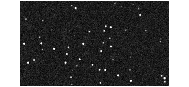
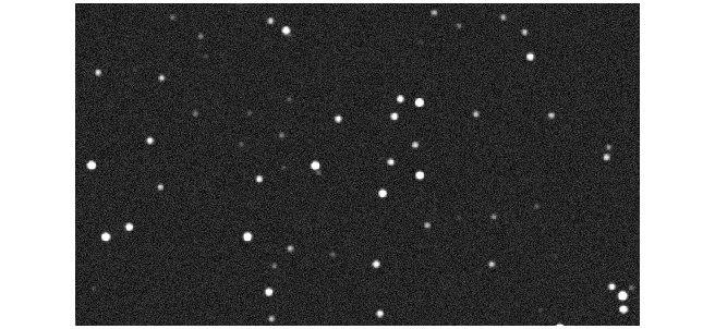
sample’s eight frames have an asteroid moving across a field of stars:
s = pc.stack("frames/", scale="asinh", limits="99.5", height=480)
The maximum through the frames shows where the asteroid went, a dot for each frame:
s.set_view(collapse={"stat": "max"})
Image(s.snapshot())
The median through the frames leaves it out, and keeps the stars with less noise than any one frame:
s.set_view(collapse={"stat": "median"})
Image(s.snapshot())
"from" and "to" (frames from 1) collapse only some of the frames, and every statistic is in
pc.COLLAPSE_STATS: mean, median, sum, std, min, max, and along the cube’s axis
moment0, moment1 and slope. collapse=False shows single frames again:
s.set_view(collapse=False)
now = s.set_view(frame=3)
now["image"]["frame"]
{'n': 3, 'of': 8, 'kind': 'file or HDU'}
Which viewers answer#
A command that changes the view can go to any viewer, even one not on screen yet; a command that reads from it needs a viewer that can answer while your code runs.
A viewer connected directly answers: a pop-up window, a browser tab, and a notebook viewer with a green dot under it (through jupyter-server-proxy, or with the browser on the same machine; see Running on a server).
A viewer not shown yet takes a change when it is shown. In the same cell as
pc.show, the viewer isn’t on screen yet, so a change waits for it and givesNone:
w = pc.show("night2.fits")
w.set_display(colormap="viridis")   # None: made when the viewer shows its image
A notebook viewer reached only through the kernel (the amber dot) takes changes at once, but can’t answer while a cell runs: the methods that read say so, and
w.tab_urlopens the same view in a browser tab that can.
In VS Code or the desktop app#
pc.popup(data, where="editor") shows the data in the Pixel Clarity already open in VS Code or the
desktop app on the same machine, instead of a browser tab. Turn on its Remote control setting
first (pixelClarity.remoteControl.enabled; in VS Code, in a window where Pixel Clarity has been
used). Over SSH it needs no forwarded port: your script and the editor’s side of Pixel Clarity are
on the same machine.
import pixel_clarity as pc

for frame in camera:                                   # your frames, as arrays
    v = pc.popup(frame, where="editor", window="camera")
print(v.region_stats("image; box(512,512,100,100)"))
Each call with the same window writes over the same file, and the view reloads with its zoom,
stretch and regions as they are. The view it returns has the methods on this page, and every one
of them answers. Where no Pixel Clarity is listening, pc.popup opens a browser tab as usual, with
a line saying so.
From the viewer to code#
Right-click the image and choose Copy as Python… to get these calls for what you did by hand. Your steps is one call per step, in order: the stretch and colors you set, the regions you added, the view you turned, with a comment where no command can do it yet (a mosaic’s levels, a crop). This view exactly opens the view as it is now, from its saved state. Paste either into a cell to do it again, on this data or on the next.